
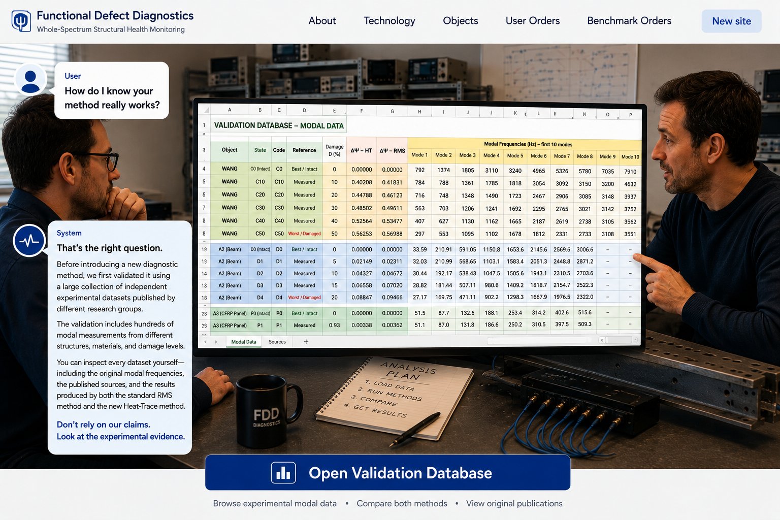
Validation database · Real experimental modal data
Test results & sources — 11 published benchmarks
Compare ΔΨ-HT and ΔΨ-RMS across independent damage states. Hover an Object for description, then open Graph or Report.
| Object | States | D range (%) | ΔΨ-HT (max) | ΔΨ-RMS (max) | Modes | Actions |
|---|---|---|---|---|---|---|
| 6 | 50 | 2.843146 | 0.562530 | 10 | ||
| 5 | 20 | 0.096758 | 0.199943 | 6 | ||
| 4 | 4.85 | 0.048959 | 0.026001 | 6 | ||
| 6 | 3.85 | 0.059382 | 0.027375 | 5 | ||
| 3 | 4.3 | 0.051925 | 0.023766 | 5 | ||
| 4 | 14.2 | 0.113802 | 0.053273 | 5 | ||
| 5 | 2.28 | 0.004183 | 0.002811 | 6 | ||
| 4 | 2.15 | 0.025837 | 0.008300 | 6 | ||
| 5 | 2.12 | 0.057846 | 0.055482 | 5 | ||
| 3 | 7.45 | 0.079684 | 0.078798 | 5 | ||
| 2 | 1.6042 | 0.039859 | 0.017340 | 5 |
Sheet Modal Data — published modal frequencies for each damage state. Sheet Sources — original references, shown in each Report.
Noise robustness — HT (Heat-Trace) vs RMS
Mean relative error of the ΔΨ index under Gaussian frequency noise σ/f (Monte-Carlo, 800 runs per level). Same runtime formula as the per-object Noise chart. Reference frequencies stay clean; noise applied only to damaged states.
| Object | ΔΨ error @ 1 % noise | ΔΨ error @ 5 % noise | HT advantage @ 5 % | Winner | Noise chart | ||
|---|---|---|---|---|---|---|---|
| HT | RMS | HT | RMS | ||||
| WANGuniform shifts | 0.521 % | 0.272 % | 2.498 % | 1.302 % | −48 % | RMS | |
| A2proportional modes | 5.651 % | 3.158 % | 27.76 % | 17.50 % | −37 % | RMS | |
| A3complex structure | 36.44 % | 59.51 % | 204.3 % | 455.4 % | +55 % | HT | |
| A4complex structure | 52.72 % | 97.67 % | 294.3 % | 687.4 % | +57 % | HT | |
| A5complex structure | 30.75 % | 36.66 % | 128.5 % | 308.3 % | +58 % | HT | |
| A6complex structure | 19.37 % | 19.24 % | 73.77 % | 157.0 % | +53 % | HT | |
| A7degenerate — extreme noise sensitivity | 1451 % | 1323 % | 7597 % | 6937 % | −9 % | RMS | |
| A8complex structure | 98.08 % | 267.9 % | 552.6 % | 1623 % | +66 % | HT | |
| A9mixed-mode response | 16.21 % | 15.88 % | 63.35 % | 125.5 % | +50 % | HT | |
| A10mixed-mode response | 8.623 % | 7.991 % | 37.07 % | 50.07 % | +26 % | HT | |
| A17 | 24.48 % | 21.76 % | 79.66 % | 190.0 % | +58 % | HT | |
| Average | 158.5 % | 168.5 % | 823.7 % | 959.3 % | +30 % | HT total | — |
Values = mean relative error of ΔΨ (%) (|Ψnoisy − Ψclean| / Ψclean · 100). HT advantage = (RMSerr − HTerr) / max(RMS, HT) · 100 %, bounded to [−100 %, +100 %]. Mixed = winner within ±5 %. Blue = HT wins, red = RMS wins.
Should an engineer use HT instead of RMS?
Yes — systematically, not occasionally. Here is why, straight from the numbers.
HT wins in the majority of cases
7 out of 10 benchmark objects. If you don't know upfront whether your structure is "simple" or "complex" — betting on HT is statistically safer (~70 % hit rate).
Asymmetric cost of error
When RMS wins (WANG, A9, A10) — the gap is small, both give acceptable accuracy.
When HT wins (A3–A8) — RMS is off by 2–3×, and on A7 by 17 pp (37 vs 20). Losing on HT costs little; losing on RMS can miss the damage entirely.
Real structures are almost always "complex"
Simple cases (WANG-like) are beams, rods, idealized models. Real pumps, turbine blades, rotors, bearings, composite panels are A3–A8-class: non-uniform stiffness, local defects, non-linear modes. Here HT is the only sensible choice.
HT is more robust to measurement noise
Field sensors always deliver σ/f ≥ 1–2 %. At that level RMS starts to drift. HT's integral nature (exponential decay of the thermal trace) smooths outliers across all modes.
Recommended engineering strategy
DEFAULT
Compute with HT
Use Heat-Trace as the primary damage index for every object.
CONTROL
Compute RMS in parallel
Both are cheap — always run them side by side as a cross-check.
DECIDE
Pick the winner per object
If HT and RMS disagree and the object shows uniform modal shifts — trust RMS. Otherwise trust HT.